Elo Rating

The Elo rating system, pronounced EE-loo, was invented by the Hungarian/American physicist, Arpad Elo in the 1950s. This system is widely used in chess and other sports to produce a scaled rating of player or team abilities. These ratings are calculated according to the expected outcome between two sides given their current rating values. These expectations, in turn, are found by determining the log-odds of each player winning the match given a scaling factor of 400. The result of the scaling is that a player with a rating 400 greater than her opponent is ten time more likely to win than the other way around. When the probability of winning is plotted versus difference in rating scores, we get the graph shown below.

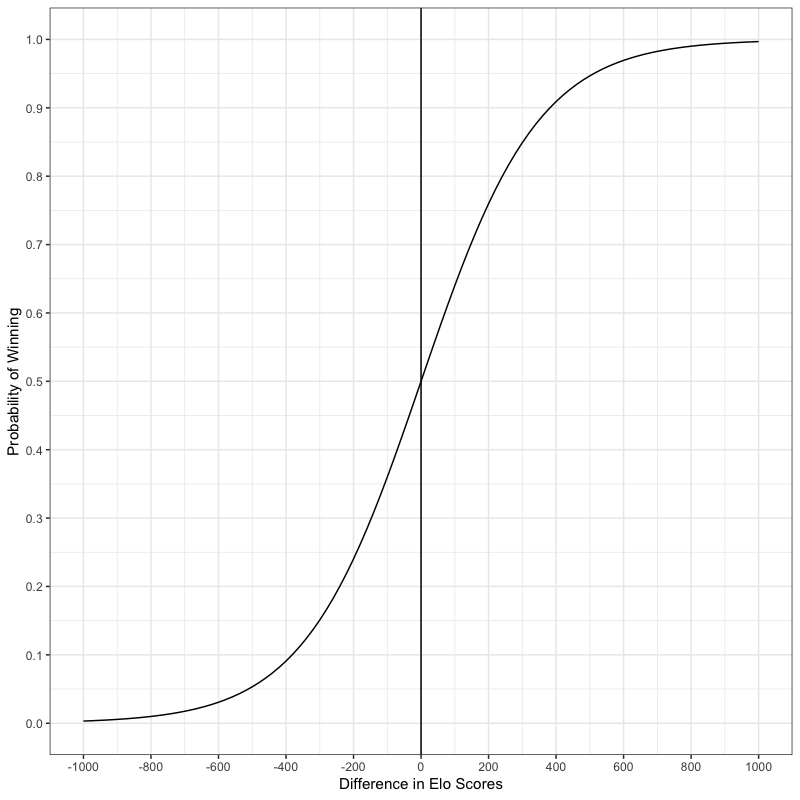
This is a logistic curve with an inflection point at where each player has the same rating. I made this plot using R. If you would like to make it too or modify it in some way, here is the code that I used.

#######################################################
## Code to Generate the Elo graph
##
## © Dr. Clifton Franklund
## MIT, 2019
#######################################################

library(ggplot2)

myFunction <- function(x) 10^(x/400)/(1+10^(x/400))

png("Elo_plot.png", width=800, height=800, res=100)
basePlot <- ggplot(data.frame(x = c(-1000, 1000)), aes(x))
basePlot + scale_x_continuous(breaks=seq(-1000,1000,200)) +
	scale_y_continuous(breaks=seq(0,1,0.1)) +
	stat_function(fun = myFunction) +
	xlab("Difference in Elo Scores") +
	ylab("Probability of Winning") +
	geom_vline(xintercept = 0) +
	theme_bw()
dev.off()

We can calculate the expected probability of a player as follows. Let’s assume for example that we have a chess game between two players with ratings R.

The first thing that we need to do is transform the player ratings into a scaled value, T. We can accomplish this with this formula: $ T=10^{(\frac{R}{400})} $. So for our example players we would get:

Now the expected winning probabilities for the players can be found by determining the log-odds. That is the calculated as $ E_{1} = \frac{T_{1}}{T_{1} + T_{2}} $. In our example, this would lead to:

The actual result of the game can only take on one of three values, 1 for a win, 0.5 for a draw, and 0 for a loss. Therefore, if player 2 wins or draws they will be outperforming their expected score. Player 1, in contrast, would need to win to outperform their expected score. Let us assume the most probable result occurs and the scores, S, are as follows:

The fact that the actual scores and expected scores do not match can be taken as evidence that the players’ current ratings are not accurate representations of their abilities. Thus, we will want to adjust the original ratings to consider our new game data. This is performed by comparing the actual and expected scores and altering the original rating by the difference multiplied by a scaling factor called the K-factor. The USCF and our club use the value of 32 for the K-factor. Larger K-factors make the adjusted scores move faster and smaller K-factors have less pronounced effects upon the adjustments. The formula for a revised score is given by $ R’ = R + K \times (S - E) $. In our example, this would be:

The more improbable the actual result is, the bigger the adjustment made to the original score. This is how all of our club scores are calculated and reported.